https://www.usenix.org/conference/osdi18/presentation/moritz
Team members: Rodrigo Castellon, Trevor Leon, Russell Tran
Code: https://github.com/rodrigo-castellon/babyray
Introduction
This paper provides a single unified system for running distributed machine learning and reinforcement learning (ML/RL) workloads. Previous systems in the literature only accounted for partial components of the entire distributed ML/RL training and serving workflow, which would be cumbersome to stitch together. For example, Tensorflow/PyTorch can facilitate distributed training, but do not support distributed serving or simulation. Other systems like MapReduce or Spark are overly focused on homogeneous distributed computation, and do not lend themselves naturally to the heterogeneous, dynamic, fine-grained computations found in RL training. Ray provides an easy to use and complete system for the entire RL pipeline that requires minimal code changes. Some key feature highlights of Ray that make it suited for RL workloads include distributed futures and bottom-up scheduling.
Results We Chose
Figure 8a, Figure 9, Figure 10b.
To properly scope this project, we decided to avoid targeting any machine learning-related features. We limited our scope to the microbenchmarks as detailed in section 5.1 of the paper. We picked these three specific figures because they were both achievable but still required nontrivial features in the Ray architecture to be implemented (futures system, locality-aware scheduling, GCS disk flushing, etc.), as well as capturing the quantitative measurements of the Ray system, which is ultimately what determines its viability.
Ray Architecture
Ray is implemented in ~40k lines of C++ and Python. A short overview of the system design that is relevant to our replication effort:
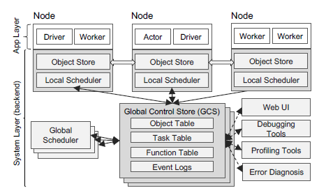
Each node contains an application and system layer. The application layer is responsible for running user code, while the system layer controls data inputs and distributed scheduling. At the local level, the Object Store stores the object data for all of the objects stored on the node, and the Local Scheduler determines if a given task is runnable on the node due to hardware constraints or too many previously scheduled tasks. At the GCS, the Object Table is responsible for storing object locations and metadata, the Task Table stores data for task repeatability, and the Function Table records remote functions that have been registered with the system. The Global Scheduler is responsible for scheduling tasks on to Workers when a Local Scheduler has determined that a local node cannot handle that task. The system implements a variety of strategies for managing fault tolerance, including chain replication of the GCS, task reconstruction when a node perishes, and flushing of all metadata in order to ensure system wide tolerance.
Our Methodology
Core Architecture and Design
We implement Baby Ray, a distributed system that contains the same core architecture and exposes the same API as Ray, in ~10k lines of Go and Python. We use Docker Compose to simulate our Baby Ray cluster on a single laptop. We chose this approach rather than the original one in order to facilitate faster development and testing. We design details of the architecture not fully described in the original paper from scratch. For example, we design a protocol with gRPC to emulate the message-passing behaviors described in the original paper, and we implement a `babyray` Python package to expose the same client API. We do not implement any of the front-end features of Ray, as they were not pertinent to replicating the results we sought, nor do we implement the “actor” model of stateful computation, as it seemed too tall a task for this project.
Figure 8a
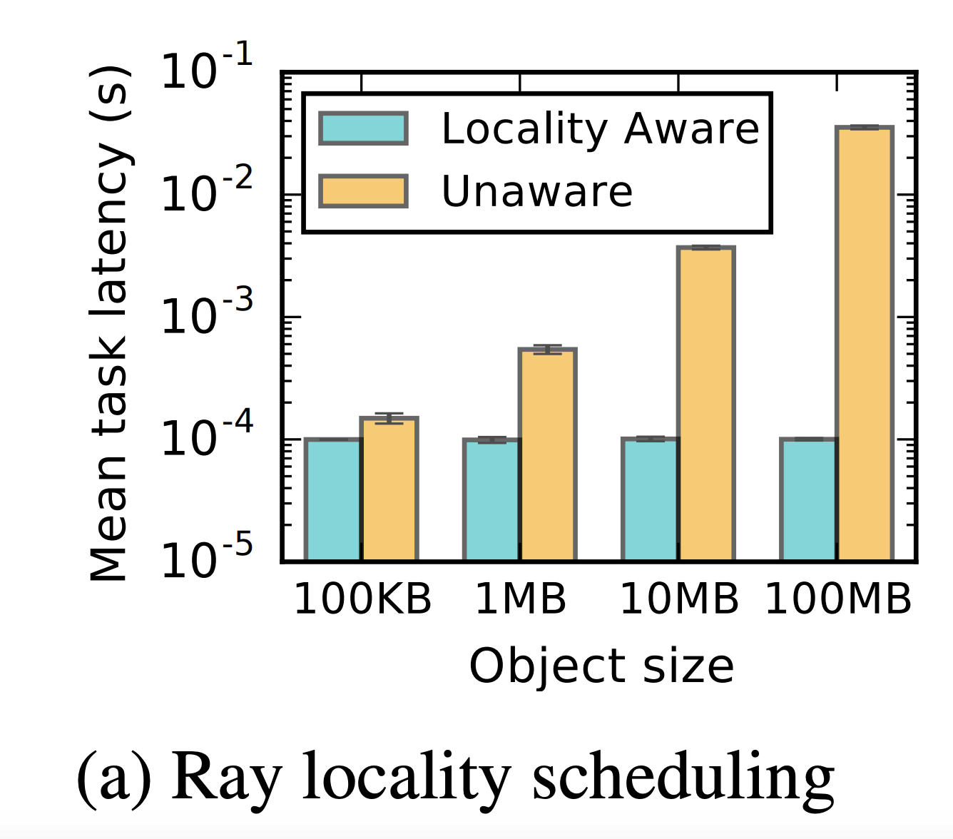
Figure 8a demonstrates the utility of locality-aware scheduling in the Ray architecture. Locality-aware scheduling refers to the idea that if we have a Ray task that depends on objects stored on Ray worker nodes, then the scheduler should attempt to schedule the task onto nodes that contain those inputs. More specifically, the scheduler actually calculates the estimated waiting time for a particular task for every worker node in the cluster (sum of queueing time and input data transfer time), and schedules where the worker will wait the least amount of time.
As described in the paper:
Tasks leverage locality-aware placement. 1000 tasks with a random object dependency are scheduled onto one of two nodes. With locality-aware policy, task latency remains independent of the size of task inputs instead of growing by 1-2 orders of magnitude
Figure 8a shows as much, that in this simple setting task latency (which we interpret to be how long it takes from the client-side scheduling call to the completion of the function execution) scales with object size if tasks are located only according to queue waiting time, but that the task latency is constant if tasks are located according to data locality.
Figure 9
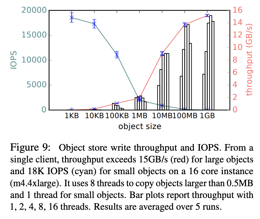
Figure 9 focuses on a single local object store’s writing throughput performance. The authors test writing data of varying sizes to the local object store and measure both the input/output operations per second (IOPS) and the overall write throughput. It is unclear to us whether IOPS refers to reads and writes or just writes, but we assume for simplicity the authors ran only write tasks.
The authors find that the object store IOPS and throughput behave as expected: larger objects always tend to take longer to move back and forth (lower IOPS), but they have a comparatively higher throughput. Notably, they find that throughput exceeds 15GB/s for a single client for large objects.
Figure 10b
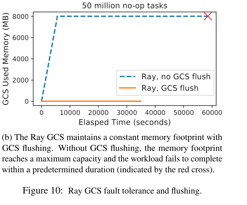
Figure 10b showcases the flushing functionality of the Global Control Store (GCS), the set of nodes responsible for keeping track of metadata such as task lineage, object locations, and the function registry. To corroborate this functionality, the figure plots memory consumption for the GCS with and without flushing, and shows that flushing to disk effectively keeps memory consumption to minimal levels throughout task execution, whereas lack of flushing leads to memory bloat.
Unfortunately, the paper omits details about how flushing is actually implemented. Correspondence with the original authors suggests that the authors leveraged Redis’s append-only file flushing feature, but the mechanism by which the system actually resolves cache misses remains unclear.
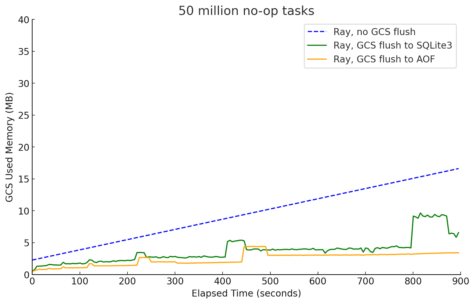
We implement both a Redis-backed disk flushing mechanism (without cache miss handling), following the original paper, as well as a SQL-based disk flushing mechanism (with cache miss handling), to provide full functionality. We follow the paper and similarly submit a stream of empty tasks and plot the memory consumption of the GCS over time under these three settings.
Results We Obtained
Figure 8a
We fail to fully replicate this figure. As shown below, as object size increases 100KB to 100MB, the locality-unaware tasks indeed take much longer to complete, as expected. However, the locality-aware task execution time still experiences some minor adverse scaling before the 100MB regime and explodes on 100MB objects. In addition to these discrepancies in relative magnitudes between locality-aware and unaware task execution times, we also see a ~100x slowdown in absolute magnitude (1E-4 -> 1E-2 for 100KB objects for example).
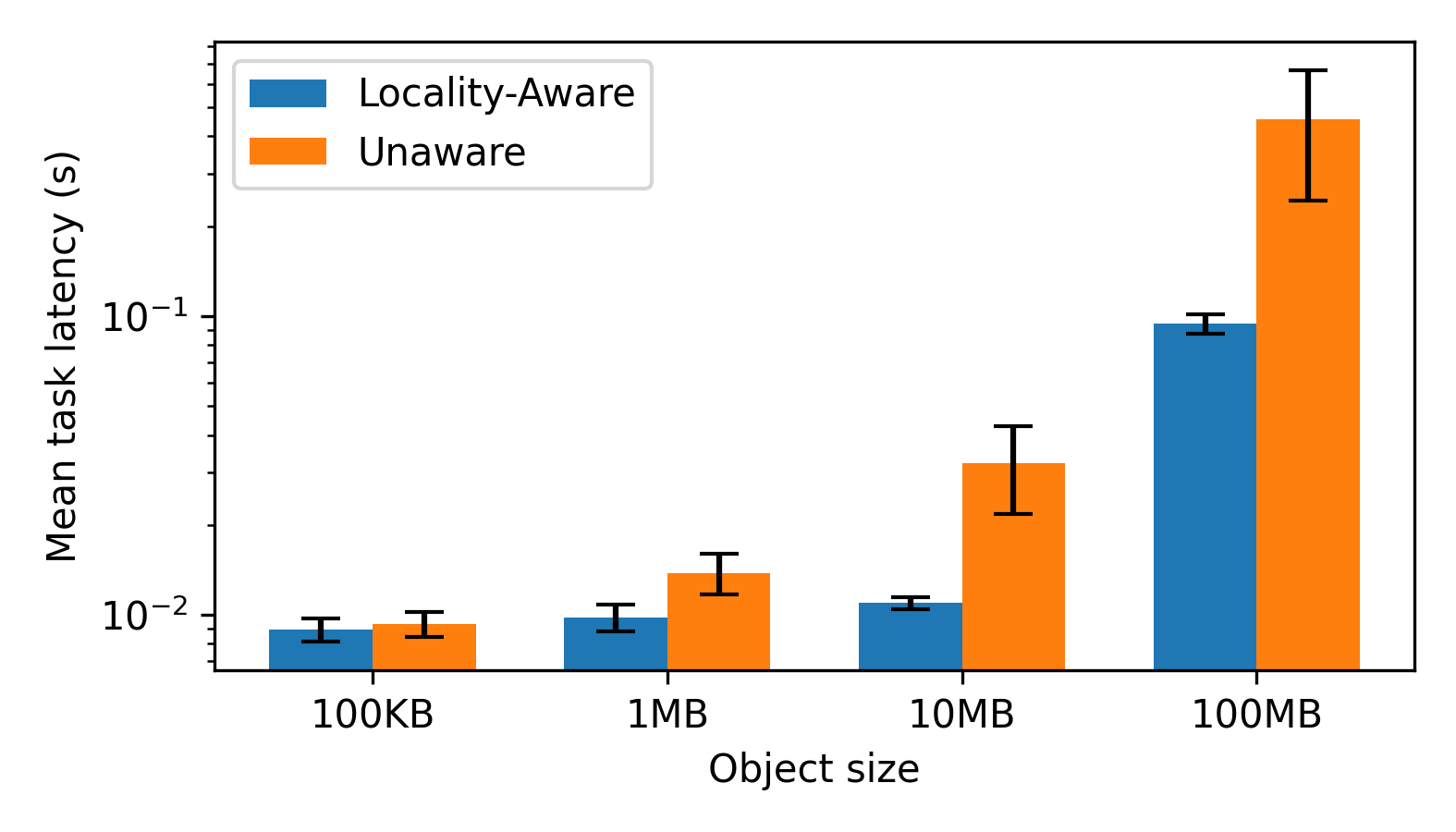
For the relative magnitude discrepancies, we believe that the data-fetching step contains a hidden processing step that scales with object size, which we have yet to discover.
For the absolute performance discrepancies, there are two obvious potential factors at play:
- Hardware mismatch. We run our experiments on a 2022 M2 Macbook Pro, whereas the authors run their CPU experiments on m4.16xlarge CPU instances on AWS.
- Software stack mismatch. Our implementation is in Golang, whereas Ray uses C++.
However, we believe the most likely factor is the difference in time investment in system optimization. For a full explanation, see our dedicated section on this.
Figure 9
We fail to fully replicate this figure as well. While the general trend is similar—as we increase the sizes of the objects we write to the local object store, the throughput generally increases and the IOPS generally decreases—, the absolute magnitudes are off by a significant margin and the curves have some counterintuitive behaviors at the extremes.
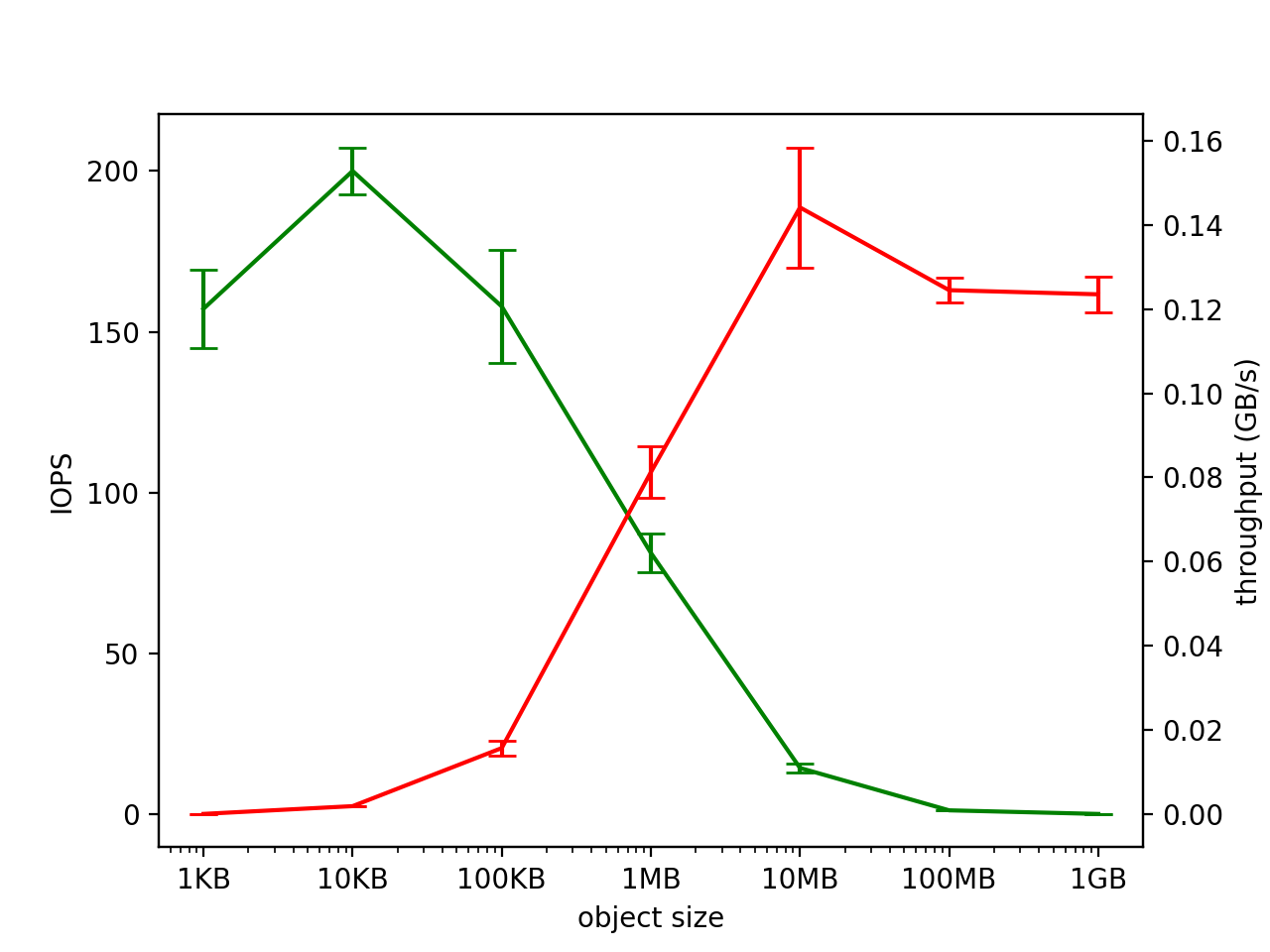
We don’t have great hypotheses for the discrepancies in the curve shapes. As for the absolute discrepancies (e.g., we achieve only ~0.15GB/s throughput whereas the authors achieve 15GB/s throughput), we again largely attribute this to reduced focus and time on systems optimization. See the subsection in the discussion on this for a full explanation.
Figure 10b
We also fail to fully replicate this figure. While the original figure shows straight piecewise curves, ours is quite irregular. We attribute this to temporary memory allocations, although an in-depth memory profiling would be necessary to confirm this.
Discussion
Systems Optimization
We believe that the absolute performance differences between our system and the original Ray system can be largely attributed to the amount of expertise, time, and effort that has been dedicated towards low-level optimizations between both systems.
We have allocated most of our limited time to building a functional architecture, dedicating much less time to improving its performance to match absolute numbers. Despite this, the few systems optimizations we have implemented have been extremely impactful. For example, rewriting the worker server from Golang to Python, which took about 5 hours of engineering time, resulted in a roughly 10x performance speedup*.
Given the impactful results from this single optimization, it stands to reason that many low-hanging fruits still exist to further optimize Baby Ray. To put our project into perspective, our 7-week sprint pales in comparison to the Ray team’s two-year full-time effort leading up to their OSDI 2018 publication. Therefore, we believe with additional time and effort, it should be possible to close the gap to the original results.
*Early on we were puzzled why empty tasks took ~70ms to execute. While we initially hypothesized that unoptimized gRPC overhead was likely the contributing factor, we profiled our code and discovered that ~60ms was contributed just by the worker server executing the empty Python function. It turned out that incredible overhead is added from on-demand spinning up Python execution environments in Go. To eliminate this overhead, we rewrote the entire Go worker server in Python, resulting in ~5ms execution times, a >10x performance improvement.
Lessons Learned & Challenges
System Design
One of the key lessons we took away from the first few papers we read in class is that often the most successful networking projects prioritize the “move fast and break things” / “organic bottom-up” philosophy. Throughout this project, we’ve seen first-hand echoes of all of these related ideas. We spent the beginning of the project trying to lay out the gRPC protocol in a top-down fashion, a deceptively challenging undertaking as there were many small yet significant details we could not foresee. We quickly transitioned from this approach to tracing through a toy example execution and defining protocol method signatures and implementations as needed in pseudocode, which was much more effective. We also learned the importance of code coverage in our unit tests, which was something that really helped us to iterate quickly.
Synchronization
One thing that trying to create a distributed system on this scale taught us very quickly was the difficulty inherent to synchronization and coordination. There are no doubt still race conditions that exist in our implementation, and it seems like it would take a significant testing effort to bulletproof a system this complex. We hope that this project could serve as a smaller-scale example for reasoning about distributed systems, since it is much simpler and easier to parse than the entire Ray implementation.
Python’s Dynamic Nature
Since Python is difficult to statically analyze, this created a lot of challenges. For example, we were never able to achieve remote recursion on Baby Ray. This is due to some technical reasons with a function in Python being unable to resolve the expression corresponding to the decorated version of itself. In fact, Python was unable to resolve any expressions corresponding to the decorated versions of functions initialized and decorated after the given remote function in the execution.
Instructions to replicate
For the full instructions see the README. Briefly,
- Clone the github repository, https://github.com/rodrigo-castellon/babyray/
- Check out the right commit corresponding to the figure you want to replicate. For example:
- Figure 8a: 7af69d3eb4147e3d5bbc7ee89c0656721c39809a
- Figure 9: 34e4dc69b473d424fedf044ca1a6ef25f5e74a47
- Figure 10b:
- No flushing: 55d7300226d232514df47fc9f22193b649786fb7
- Flush to MySQL: 192b4ef4905101fdde56aa768c40b9fa2d2e5a62
- Flush to AOF: e070c8b31f9bcc74f8a138c60c94fef56a3e9cf3
- Run make docker
- Then run ./scripts/run_fig{number here}.sh, corresponding to the figure you would like to replicate.
- Dump the right logs:
- Figure 8a: docker-compose logs worker1 | grep time > log.txt
- Figure 9: docker-compose logs worker1 | grep RES: > log.txt
- Figure 10b: docker-compose logs gcs
