CS244 ’13: Increasing TCP’s Initial Congestion Window

Group: Kyle Brogle, Lavanya Jose

Introduction:

In the paper “An Argument for Increasing TCP’s Initial Congestion Window”, the authors argue that increasing the TCP initial congestion window init_cwnd to ten segments from its typical 3 segments used in practice.  They believe that this will decrease latency of connections, and allow short transfers to compete fairly with bulk data traffic, among other things.  The authors validate the claims of decreased latency by experimenting with different init_cwnd values in a live test on the Google Search infrastructure.

What makes this problem interesting is that idea that one small parameter change in TCP can cause a large improvement in the performance seen by the protocol, both in terms of completion time, and to a lesser degree, fairness to short flows.  Furthermore, such a change is easy to implement, as it can be done on a per-server basis, and doesn’t require changes to clients (assuming that the client’s receive window is large enough to see benefits from the change).

We replicated these results from figures 5 and 7 using emulated hosts in Mininet.  Using a platform such as Mininet instead of a large-scale production test will give us finer control over bandwidth and round-trip time, which were estimated in the experiment by computing a running average of link throughput for bandwidth, and taking the minimum round-trip time.  Also, as described below in our results section, using emulated hosts in Mininet instead of data from production servers, allows us to fix all but one variable in the experiment when running tests.  This allows us to more easily interpret the results we obtain.

Configuration:

For our experiment, we use a simple topology with two clients and one server connected to the switch.  Instead of using running averages of link throughput and round-trip time, we set these directly by configuring the relevant properties (delay, bandwidth) of the links.  We use Python’s built-in SimpleHTTPServer class on the server in order to serve static webpages.  On the client, we use wget in order to retrieve webpages.  We use the “ip route” command to modify init_cwnd on the server and init_rwnd on the client, as the paper notes that init_rwnd must be set at least as high as the new init_cwnd value, as the window size used is the minimum of the two.

Verifying our Configuration:

In order to verify our configuration, we first test test the latency and bandwidth of the links using ping and iperf, in the same manner as in assignments one and two.  We then verify that we are able to successfully set init_cwnd and init_rwnd values on our Mininet hosts.  In order to do this, we reconfigure the server’s init_cwnd and the client’s init_rwnd, and have the client fetch a static page from the server.  We use the tcpprobe kernel module to inspect the cwnd value for the packets in the flow, confirming that the first packet sent by the server in the flow seen has the correct cwnd.  In the figure below, we have changed the init_cwnd to 20 segments and use tcp_probe to plot the evolution of the cwnd while a mininet client fetches a page from a webserver.  This was our initial method of verifying our ability to set init_cwnd.

Results:

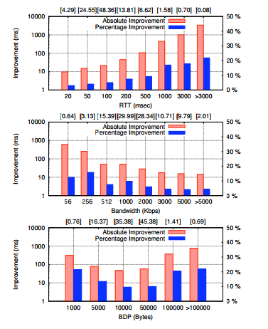
Figure 5 from the paper

Figure 7 from the paper

Above are the selected graphs from the paper (figures 5 and 7) as well as our reproduced results.  Our RTT graph is very similar to the RTT graph found in the paper, with absolute improvement growing as RTT increases.  This makes sense, as the savings provided by increasing initcwnd should be constant in the number of round trips.  The main difference between our RTT plot and the paper’s is that we report no improvement for an RTT of 20ms.  We believe this is due to a fundamental difference between our experiment and the paper’s.  In the paper, the authors use sample data collected from production servers, and bucket the results.  This means that when measuring RTT for instance, they do not control for bandwidth.  The paper states that high BDPs should see the most improvement, since responses with size greater than the BDP need multiple RTTs regardless of the value of initcwnd.  In general, connections that have such a low RTT tend to have high bandwidth, so it is likely that the 20ms measurement from the paper has connections with higher BDP than our tests (with default bandwidth equal to 1.2Mbps).  In our measured example, an RTT of 20ms causes the response size to be greater than BDP, offering no improvement with larger initcwnd.

For the author’s bandwidth graph, the absolute improvements decrease as bandwidth increases.  For Mininet with a 70ms RTT, the lower two bandwidth buckets hardly show improvements. The authors see improvements because their low bandwidth networks likely have high delays, allowing them to send more bytes per RTT with cwnd=10. In our case with an RTT of 70ms, the BDP is less than 2.5 KB for the 256Kbps link and it becomes a bottleneck for both cwnd=3 and cwnd=10. The little improvement that is there may come from losses arising from the buffer filling up. During a loss the cwnd drops multiplicatively (eventually below the BDP), in which case cwnd=3 is more limiting than cwnd=10.

We verified that increasing the delay to 343ms (the median latency for their low bandwidth links) shows higher improvements for low bandwidth links, since now for cwnd=10, 10 segments can fit on the link in 1 RTT.

The bandwidth graph recomputed with an RTT of 343ms.

Our BDP graph differs from the paper’s graph mostly in the lower 2 bars (for BDPs 1000 and 5000).  Where the paper shows improvement in these buckets, our measurements show very little improvement.  Seeing little improvement here makes sense, as if the response size is larger than the BDP, we won’t see as much improvement.  This is explained in the paper, and is because a higher BDP allows more bytes to fit in the link per RTT, causing smaller response sizes to never leave the slow start phase of TCP.  The improvement show in the paper for these low BDPs then is likely due to some effect of higher initcwnd other than a savings with higher BDPs.  The paper lists other advantages of a larger initial window size, including better fairness for short transfers and faster recovery from losses.  If the responses in the paper’s measurements for these buckets are small, the improvement may be due to a combination of improved fairness and higher chance of loss recovery through Fast Retransmit.

Finally for the “Latency Improvement v/s Number of segments” graph, the main discrepancy between the authors’ graph and ours is that we see huge improvements in latency for small files (3, 4 segments) while they see very little improvements.  At first it seems hard to explain, since the BDP (70ms * 1.2Mbps ~ 7 segments) is high enough for the response to be sent in one RTT for cwnd=3 and cwnd=10.  For RTT=70ms, the improvement was around 1RTT.

We checked the actual packets sent during the TCP connection using Wireshark to figure out the source of the discrepancy.  It turns out that even though the file was only 3 segments, the server also sent an additional segment containing just the HTTP OK response before sending the file.  For cwnd=3, it would send out the response and the first 2 MSS of the file in one RTT and the third MSS in the next one.  For cwnd=10, it would send the response and the whole file in one RTT (4 segments).  Thus it saved at least an RTT every with cwnd=10.  To confirm that small enough files do indeed see no improvements, we compared the latencies for files smaller than 3 segments (see figure).

Challenges:

During the design of our experiment, a few challenges stood out that gave us some trouble.  First was that when automating the validation of initcwnd, we found that the tcp_probe module would sometimes give incomplete data.  After some trial-and-error, coupled with the source code of the module, we found that the problem was that the output of tcp_probe was not being flushed from it’s kernel buffer until after our test completed.  To remedy this, we made sure to run iperf for long enough to trigger a flush of the buffer.

The other main challenge of our experiment was the lack of data concerning parameters in the paper.  Since the data used was taken from a production environment, we were often given aggregate values of parameters such as bandwidth and RTT.  Since we were controlling all variables except one in our experiment, we needed to decide, for example, how to set bandwidth and number of segments during our RTT experiment.  To decide the number of segments, we looked at measurements for the average number of segments in a query response, and set our default RTT and bandwidth parameters to match the median BDP reported in the paper, which was 10.5KB.

While Mininet was very useful in our experiment setup, allowing us to control for variables during our tests, the reproducibility of our results is very dependant on our choice of default parameters.  While we set these defaults based on the medians given in the paper, it would be interesting to extend the experiments with other default values, and observe how it affects the improvements seen from higher initcwnd values.  Historically, recommended initcwnd values have increased as BDPs have increased in the internet.  Since RTT is limited by propagation delay, this increase mostly comes from increased link bandwidth.  It would be interesting to use our experiment, with similar delay parameters but higher bandwidths, to test a range of initcwnd values, and try to determine the most effective initcwnd values for different average BDPs.

Conclusion:

Based on our experiments, we were able to confirm that increasing the initcwnd value from 3 to 10 does lead to lower response latency.  In some cases, the authors reported larger improvements than our experiments showed, likely because the authors used data collected from production servers, leading to some variables being correlated (for instance, a high bandwidth connection likely has low latency, and vice-versa).

Instructions for Reproducing:

1. Create a c1.medium AWS instance* using AMI ami-e269fcd2 in US West (Oregon), and clone our Git repository** from https://bitbucket.org/broglek/iw10
2. In the iw10 folder, execute ‘sudo ./run.sh’.  Graphs will be in a timestamped folder, labelled with the parameters used to generate them.  Note: Generating all 4 graphs can take around 3 hours.  By toggling the 4 “run” flags in run.sh to 0, you can choose to generate only certain graphs at a time (e.g. setting –run-bdp 0 will skip generating the bdp graph).

*When using our AMI, the username is ‘ubuntu’.  It is essentially the AMI given to us at the start of CS244, but with a few added comforts (such as emacs).

**If trying to use the git repository without the AMI, you will need to have Mininet (and all dependencies) installed, as well as NumPy, Matplotlib, iperf, and the tcp_probe module, and be running Linux with kernel version greater than 3.3.

Sources:

• Dukkipati, Nandita, et al. “An argument for increasing TCP’s initial congestion window.” ACM SIGCOMM Computer Communication Review 40.3 (2010): 27-33.
• Chu, Dukkipati, et al. “Increasing TCP’s Initial Window.” IETF Internet Draft (2012) http://datatracker.ietf.org/doc/draft-ietf-tcpm-initcwnd/