CS 244 ’13: Increasing the TCP Initial Congestion Window

Introduction

In [1] the authors advocate for an increase to TCP’s initial congestion window (init_cwnd). They argue that the value that most TCP flows start with (3 segments) is a value based on antiquated network speeds and that it’s time to revisit standardizing a new value for the init_cwnd. Today, the majority of TCP connections are short-lived and finish before the completion of the slow start phase, which means that an optimal value for the congestion window was likely never experienced. The results of their experiments show that using an init_cwnd value of at least 10 segments is a simple way to have a significant positive impact on Web transfer latency. In particular, they showed that increasing init_cwnd to 10 segments improved the average latency of HTTP responses by 10% with the greatest benefits for networks with high round-trip times and bandwidth delay products. In our experiments we aim to verify the improvements they see by modifying init_cwnd and to explore the question if their proposed init_cwnd value is truly optimal. In particular, we replicate their Figure 2 and Figure 5 results: “TCP latency with different init_cwnd values” and “Average response latency for web search bucket by RTT (round-trip time), BW (bandwidth), and BDP (bandwidth delay product).”

Background

Using a data center which [1] calls “AvgDC,” the paper produces the following figures:

Paper [1]’s Figure 2: TCP latency for Google search with different init_cwnd values

Paper [1]’s Figure 5a: Average response latency for Web search bucketed by RTT

Paper [1]’s Figure 5b: Average response latency for Web search bucketed by BW

Paper [1]’s Figure 5c: Average response latency for Web search bucketed by BDP

AvgDC had a median RTT of 70 ms and a median bandwidth of 1.2 Mbps. From this data, they recommend changing the default init_cwnd from 3 to 10 segments. (Notice in [1]’s Figure 2, init_cwnd of 16 is actually optimal; however, the paper suggests that using a window of 16 only yields marginal benefits over 10 and there are some downsides to using a larger initial window than necessary. See section “4.2 Negative Impact” in [1] for a discussion on this.) While we agree that an init_cwnd of 3 is indeed too small for the environment of today (and in fact, in 2011 the Linux kernel changed their initial congestion window from 3 to 10 [6]), we actually wondered if 10 was truly the best recommendation. In particular, we wanted to use values of RTT, BW and file response size that more accurately reflected recent world-wide usage statistics. Thus, unless otherwise noted, we use the following values for all of our results:

Table 1: Summary of Network Parameters

3 Mbps for bandwidth.	This is the 2012 global average connection speed as reported by Akamai in [4].
100 ms for RTT.	This is the 2012 worldwide average RTT to http://www.google.com as reported by a Google Developer Advocate in [5].
37 kilobytes for file response size.	This is the approximate response size of http://www.google.com we observed in February 2013 (using the tool Firebug).

Experimental Results

We used the values shown in Table 1 to find out if init_cwnd of 10 was a reasonable recommendation given current global network statistics for http://www.google.com. The below figure shows the download times of the curl command on a 37 kilobyte file and bandwidth of 3 Mbps, with varying initial congestion window (given in packets):

Our Figure 2 using the parameters in Table 1: TCP latency for Google search with different init_cwnd values

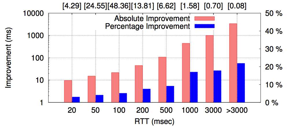
As our results show, there’s a significant benefit to raising the initial congestion window from 3 to 10. However, there’s an even greater benefit to raising it from 3 to 26 (there little to no benefit in going to 42). Thus, based on the numbers we found using statistics from 2012, we found that raising the init_cwnd from 3 to 10 yields significant benefits. The below figure shows the absolute (in pink) and percentage (in blue) improvement in changing the init_cwnd from 3 to 26 across different RTTs:

Our Figure 5a using the parameters in Table 1: Average response latency for Web search bucketed by RTT

Again, we see an even greater benefit in going to init_cwnd 3 to init_cwnd 26 (the maximum percent benefit that [1] saw was about 20% while we almost see a 40% gain in the highest bandwidths). The below figure shows the absolute (in pink) and percentage (in blue) improvement in changing the init_cwnd from 3 to 26 across different bandwidths:

Our Figure 5b using the parameters in Table 1:  Average response latency for Web search bucketed by BW

Although this does not follow the trend shown in Figure 5b in the paper, it does agree with their statement that “the largest benefits are for high RTT and high BDP networks.” We believe this is due to the fact that their data in Figure 5 is an aggregate of many different runs during their two-week long experiment. In particular, in each of these runs there will be variety of RTTs at each BW (whereas in our experiment we fixed RTT and varied BW). In fact, the paper readily admits “high BDP is mostly a consequence of high RTT paths and … we note that the percentage improvements shown in Figure 5 underestimate the attainable latency improvements.” While we could have varied RTT and BW simultaneously and plotted the bucketed results for BW here, we thought fixing RTT and varying BW better illustrated the benefits of a higher init_cwnd in higher BW networks.

Our Figure 5c using the parameters in Table 1:  Average response latency for Web search bucketed by BDP

Again, although this does not follow the trend shown in Figure 5c in the paper, it does agree with the fact that the greatest gains are seen for networks with high RTT and high BW. In the above graph, because the paper was not particularly descriptive of how they specific RTTs and BWs for each BDP, we fixed RTT at 1000 ms, and varied BW from 0.008, 0.04, 0.08, 0.4, and 0.8 Mbps to yield BDPs of 100, 5000, 10000, 50000, and 10000. We would have appreciated if the paper was a little clearer on how they obtained this graph. Even better would be for them to post the data points that generated this graph. While we could have tailored our values of RTT and BW to reverse engineer the graph they got for Figure 5c, we didn’t think this would be a particularly useful exercise. Instead, following the guideline in the paper that the greatest benefits are seen for high RTT and high BW networks, we used a fixed, high RTT, and varied BW to obtain the BDPs in the x-axis of their graph.

Conclusion

Using parameters based on current (2012) network characteristics, we replicate the trends that the authors in [1] found. The paper was written in 2010, and as bandwidth availability increases every year, we discovered that in using 2012 values, an even larger init_cwnd of 26 yields significant decreases in latency. As everyone’s network environment differs, in addition to the recommendation for increasing the default value of init_cwnd, we argue that init_cwnd should also be a dynamic value based on current network parameters. Lastly, like the authors in [1] warned, there is of course an associated cost with increasing init_cwnd. In particular, latency can increase when a higher value of init_cwnd leads to overflowing bottleneck buffers. (In fact, we actually saw such an increase when we initially forgot to turn off iperf before running another experiment.) This furthers our argument that applications should be able to tune init_cwnd based on the type of traffic they expect to send.

Appendix A: Experimental Setup

We use an Amazon EC2 instance and the Mininet network emulator to conduct our experiments. The EC2 instance was used so that we can easily manipulate available CPU and memory needed (via different instance types) and it will also be used as a way to easily share our results with our peers.

Table 2 Environment Summary

Linux Kernel	Version 3.5.0-21
Mininet	Version 2.0.0
Python	Version 2.7.3
Amazon EC2 Instance	Type c1.xlarge

In Mininet we created a simple emulated topology of a client, server and switch:

except in the experiments where we are varying RTT, BW or BDP respectively, the RTT and BW is as described in Table 1. Links in Mininet are by default bidirectional. We evenly split the delay among the links (thus, each link gets a delay of RTT/4). Our server is based on the Python module SimpleHTTPServer. We modified init_cwnd and init_rwnd using the same Linux command specified in [1], ip route, using instructions as described in [2] and [3]. We verified our topology using iperf for bandwidth, ping for latency and the Linux kernel module tcp_probe for congestion window. Note: Even though we verify bandwidth, latency and init_cwnd, because the entire experiment takes so long to run, we do not kill the experiment if any of these values differ from the expected values. Instead, we print to stdout an error message and notify the user of what the desired and actual values were. We want the user to have control of whether or not the topology was accurate enough for their experiments, and in the case where only one experiment went astray, the user can simply discard that data set, and rerun just that one experiment rather than the whole series. We created files of a specific size using the Linux command dd. We obtained web page retrieval times by using the curl command. To match the environment of [1], we also set our TCP congestion control algorithm to CUBIC.

Appendix B: Replicating Our Experiment

To replicate our experiment, create a new Amazon EC2 c1.xlarge instance using the image “CS244-Win13-Mininet.” (If you need instructions on how to make a new instance, you can consult this document: http://www.stanford.edu/class/cs244/2013/ec2.html.) Verify the versions of Linux and necessary software listed in Table 2. Clone our repo: git clone https://nicolekeala@bitbucket.org/nicolekeala/cs244_initcwnd_finalresults.git. Invoke sudo ./run.sh at the command line to run the experiments for, and to generate figures 2, and 5a through 5c. To view the data sets and graphs, change the current directory to “results.” (The “results” directory is where the csv and png files are generated.) An easy way to view png files on an EC2 instance is to run python -m SimpleHTTPServer and then inside of a browser, go to http://instance_ip_address:8000. For example, if your EC2 instance IP address is ec2-123-456-789-000.us-west-2.compute.amazonaws.com, go to http://ec2-123-456-789-000.us-west-2.compute.amazonaws.com:8000. Please note it takes about an hour to run run.sh to completion. (If desired, one can easily comment out the various scripts that run.sh calls to generate only one figure at a time.)

Appendix C: A Note on Challenges

While there were no particularly irksome challenges we experienced in our efforts to replicate and expand upon the results of [1], there were some issues that we’d like to share with future users of similar setups.

Notes on Mininet: Mininet can sometimes act in unpredictable ways if something fails mid-way through the experiment or the topology is not properly cleaned-up. Thus, as a sanity check, we ran sudo mn -c before each experiment that used a new topology (and of course, whenever we use a new topology we always verify the BW, RTT, and init_cwnd). When something really bad happens in Mininet, and sudo mn -c does not appear to solve the problem, we found the only recourse was to restart our instance.

Notes on tcp_probe: Although we eventually got it to work, we had great difficulty in initially getting tcp_probe to work for us (in particular, we’re using it to verify init_cwnd). There’s a surprising lack of examples and documentation on tcp_probe. However, the source code can be found online [7], and we found that to be an invaluable tool when trying to configure tcp_probe.

Notes on ip route: While there were quite a few examples of ip route online, we did not find the man page for ip to be particularly helpful. We were very grateful to find reference document located at [2].

References

[1] Dukkipati, Nandita, et al. “An Argument for Increasing TCP’s Initial Congestion Window.” ACM SIGCOMM Computer Communication Review 40.3 (2010): 27-33.

[2] Kuznetsov, Alexey. “IP Command Reference.” Santa Monica College, 14 Apr. 1999. Web. 18 Feb. 2013. http://homepage.smc.edu/morgan_david/cs70/ip-cref.pdf.

[3] Kayan, Sajal. “Tuning Initcwnd for Optimum Performance.” CDN Planet. CDN Blog, 25 Oct. 2011. Web. 16 Feb. 2013. http://www.cdnplanet.com/blog/tune-tcp-initcwnd-for-optimum-performance.

[4] Belson, David. “The State of the Internet.” Akamai 2nd Quarter, 2012 Report 5.2 (2012).

[5] Grigorik, Ilya. “Latency: The New Web Performance Bottleneck.” Ilya Grigorik: Developer Advocate at Google. 19 July 2012. Web. 8 Mar. 2013. http://www.igvita.com/2012/07/19/latency-the-new-web-performance-bottleneck.

[6] “TCP: Increase the Initial Congestion Window.” Linux Kernel Source Tree. Git Linux Kernel Source Tree, 3 Feb. 2011. Web. 6 Mar. 2013. http://git.kernel.org/cgit/linux/kernel/git/torvalds/linux.git/commit/?id=442b9635c569fef038d5367a7acd906db4677ae1.

[7] “tcp_probe.c” /linux/net/ipv4/tcp_probe.c. Web. 2 Mar. 2013. http://www.cs.fsu.edu/~baker/devices/lxr/http/source/linux/net/ipv4/tcp_probe.c.

Contact
Nicole Tselentis can be contacted at: nicole@cs and Greg Kehoe at: gpkehoe@.