DCTCP and Queues

Team:
Tom McLaughlin and Kun Yi.

Key Results:
DCTCP’s queue-friendly behavior was replicated on the Mininet platform. DCTCP obtains full throughput as long as the ECN marking threshold K is set above a reasonable threshold. DCTCP obtains lower queue size variability than TCP-RED.

Sources:
[1] Mohammad Alizadeh, Albert Greenberg, David A. Maltz, Jitendra Padhye, Parveen Patel, Balaji Prabhakar, Sudipta Sengupta, and Murari Sridharan. 2010. Data center TCP (DCTCP). SIGCOMM Comput. Commun. Rev. 40, 4 (August 2010), 63-74.

[2] Bob Lantz, Brandon Heller, and Nick McKeown. 2010. A network in a laptop: rapid prototyping for software-defined networks. In Proceedings of the Ninth ACM SIGCOMM Workshop on Hot Topics in Networks (Hotnets ’10). ACM, New York, NY, USA, , Article 19 , 6 pages.

[3] S. Floyd. RED: Discussions of setting parameters.

Contacts:
Tom McLaughlin (thomasjm@stanford.edu) and Kun Yi (kunyi@stanford.edu)

Introduction:

Data center TCP (DCTCP) was first proposed in [1] as a way to improve network performance in data centers, by addressing several problems with the way TCP interacts with queues. One example given in the paper is the fact that long-running TCP “background” flows can build up large queues in intermediate switching, resulting in unnecessarily high latency for short, bursty “foreground” flows. DCTCP addresses this problem by using the existing ECN mechanism built into commodity routers, and changing the behavior of the end hosts slightly. Instead of following RFC 3168 on the use of ECN, the receiver sets the ECN-Echo flag on all ACKs being sent to the sender. The sender uses these flags to estimate the probability ‘’ that the queue is full above some threshold. When the sender experiences a loss event, it reduces its window size by an amount proportional to , rather than cutting it in half as TCP does. The result of this scheme is an algorithm which “gently” decreases the congestion window on the onset of congestion, achieving high throughput and also low queue utilization.

Reading the paper, we were interested in Figure 15 of [1]. The figure compares DCTCP to TCP-RED. Part (a) shows the lower queue utilization of DCTCP, and the part (b) shows the much noisier behavior of the queue under TCP-RED relative to DCTCP. The goal of this project is to replicate Figure 15.b, demonstrating the improved stability of DCTCP. A preliminary step along the way is to replicate Figure 1, which compares DCTCP to regular TCP showing the basic queue-friendly behavior of DCTCP. Another step is to replicate Figure 14, which shows the throughput obtained by DCTCP as you sweep the marking threshold K.

Methods:

Experimental Setup

Our experiment is run on Mininet [2], with a DCTCP-enabled kernel provided by Vimal Kumar. The setup is a star topology with a total of N hosts, where N-1 are senders and the last host is a receiver. The switch-receiver link is the bottleneck.

Validating the setup

Figure 1 (DCTCP queue behavior)

We start by replicating Figure 1, which demonstrates the small-queue size characteristics of DCTCP. In the original experiment, a bottleneck link of speed 1Gbps is used. However, Mininet cannot accurately run such a large bandwidth link. Therefore we use a link of speed 100 Mbps. The setup consists of 2 senders, 1 switch and 1 host. We start with setting RTT = 4ms, K = 20 packets, max queue size = 200. The following plots compare our result (top) with Figure 1 in [1] (bottom):

 

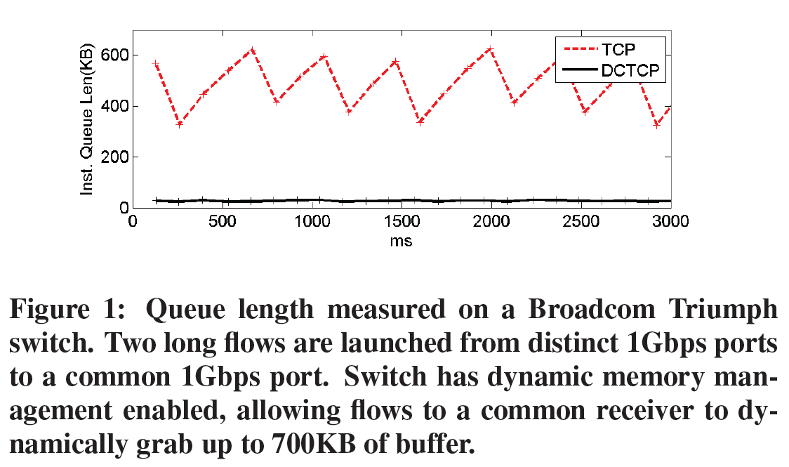
Our experiment verifies qualitatively that DCTCP works: we can clearly see that the sawtooth curve for TCP and the low queue size (around 20 packets) for DCTCP. Note that the period for TCP queue sawtooth is bigger than that in the paper. This is due to we are using operating with different settings from the DCTCP due to software constraints, and the latency in the paper’s setup is lower than what we could have used.

We notice that with a larger delay and same K, DCTCP exhibits larger variation of queue size, and spends a lot of time underflowing. This confirms the conclusion in the paper that the marking threshold has to be set properly to avoid underflow. The paper suggests derives a heuristic which suggests that the marking threshold K should be proportional to bandwidth-delay product:

However, it is also argued in the paper that the estimation is based on idealized settings, and in practice a larger marking threshold might be needed to accommodate bursts. To get the accurate minimum marking threshold that achieves full throughput, we have to sweep several values of K.

Figure 14 Replication

We decided to replicate Figure 14 from the paper in order to validate the basic workings of DCTCP. However, ECN is configured as a special case of a “red qdisc” (queueing discipline) in linux, and setting parameters of such a red qdisc has certain restrictions.

The first problem with TC-RED queues is that they don’t allow you to base ECN marking decisions on the instantaneous queue size–instead, a moving average of the queue size is kept over time, parameterized by the “burst” setting.

The second problem is that we aren’t free to choose the TC-RED parameters. They are constrained by two facts:

1. We can’t set qmin=qmax, since TC-RED needs a nonzero queue size to calculate the EWMA constant. Instead, we set qmax=qmin+1.
2. The “burst” parameters is constrained by burst>qmin/avpkt.Since the marking threshold is chosen as K=qmin/avpkt, increasing the value of K results in an an unwelcome increase in burst.

As a result, reproducing Figure 14 is not completely straightforward. The figure below (left) was created by choosing burst = 100 for all points, since then even the highest value of K will result in a successful EWMA calculation. The effect of this setting is a high weight placed on the moving average. In order to partly compensate for this, we run the experiment for long enough to reach steady-state, and we only use throughput measurements after reaching steady-state to produce the plot. The paper’s result (right) is reproduced for comparison.

Note that our tests were conducted with 100Mbps links, whereas the original paper used 10Gbps links. With these validation experiments complete, we were ready to move on to reproduce our main result: Figure 15.
Results:
In this section, we describe the experiment we performed to replicate Figure 15 (above), showing the DCTCP and RED queue size as a function of their parameters.

The paper used a testbed consisting of 94 machines in 3 racks. 80 of these machines had 1Gbps NICs, and the remaining 14 have 10Gbps NICs. Since Figure 15 was conducted at 10Gbps, we infer that they were using the latter 14 hosts. Thus, we choose N = 14 for our own setup (thirteen senders + 1 receiver). Since we want to emulate datacenter conditions, we chose the lowest delay that Mininet can support, 1ms, for the host-switch links.

The discussion in the paper says that it is difficult to set the TCP-RED parameters correctly, and we would have to agree with this. Experimentally, we find that the queue size plots are quite sensitive to RTT, as well as the number of hosts and flows used. Since Mininet must operate at much lower line rates than 10Gbps, our experiment runs in a different regime than that used in the DCTCP paper, by 2-3 orders of magnitude.

As we experimented with different settings for bandwidth, delay, and marking threshold, the most significant phenomenon we observed as a rapid increase in queue variability as the bandwidth was increased from about 50Mbps to 100Mbps. This is summarized in the figure below, showing a sweep of BW = 50, 75, and 100Mbps, with K = 2 and K = 10, delay = 1ms. (The recommended values of K using the heuristic in the paper are  0.6, 0.9, and 1.2 respectively, mainly due to the low value of C.)

We are not able to explain the sudden increase in queue variability as you increase the bandwidth, and we think it is most likely due to the fidelity of the Mininet simulation degrading at these rates. (When we ran similar tests with only N = 3 senders instead of N = 14, the queue variability was smaller, supporting this hypothesis.)

Because of our uncertainty about the higher-bandwidth conditions, we decided to conduct our Figure 15 experiment at 50 Mbps. Following the advice of the paper, K should be approximately 2 for our chosen bandwidth-delay product. The DCTCP paper recommends K be set slightly higher to account for burstiness of traffic, so we choose K = 5 for safety.

The DCTCP paper began by setting RED following the guidelines in [3], but found that RED underflowed the queue and lost throughput with these settings. As a result, they increased the RED minimum queue size under TCP achieved nearly full throughput.

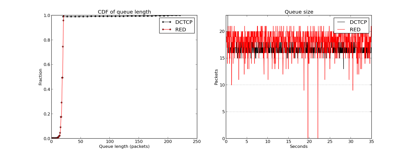
The mean queue occupancy for RED can be adjusted to reach any value by setting the minimum and maximum queue sizes. We assume that the authors chose their settings so that the RED curve overlaps the black curve in order to make comparing their relative amplitudes easier, and to compare them to each other in the low queue-size regime. The figure below shows the basic kind of results we have seen: DCTCP shows very little variation when configured with the correct value of K, whereas RED shows much higher variation. In this figure, the RED parameters are minq = 40, maxq = 80, weight = 40, burst = 40, p = 0.01.

In the spirit of the paper, we lowered the RED queue size until the two curves were almost overlapping. We were unable to get the DCTCP queue to be smaller than about 18 packets, even with the marking threshold set very low. This produced the following plot. In this figure, the RED parameters are minq = 10, maxq = 80, weight = 20, burst = 10, p = 0.01. Once again, the RED variability is higher than DCTCP.

We show one more figure below, from an experiment in a completely different regime. In this figure, N = 3 (2 senders + 1 receiver), BW = 500 Mbps, and delay = 10ms. While the correctness of the results is not certain at this bandwidth, reducing the number of senders may reduce the load on Mininet sufficiently to produce reasonable results. In this regime we set K = 70, in accordance with the usual rule. The RED settings are minq = 80, maxq = 120, weight = 40, burst = 80, p = 0.01. Both scenarios obtain near-100% throughput, although the RED scenario is on the edge of underflowing.

With this particular regime and choice of settings, the oscillation undergone by TCP-RED is clearly visible.

Our final conclusions about Figure 15 are mixed. The overall idea is certainly confirmed: in a wide variety of conditions we have tested, RED has shown about 4-10 times more queue size variability, if we measure the peak-to-peak of the queue occupancy profiles. We also conclude that the tuning of the various parameters, the number of hosts and flows, and the network delay and latency all interact to create a variety of queue behaviors, especially when the settings for DCTCP or RED are not chosen correctly. In the end, we feel we cannot accurately replicate the specific result of Figure 15, due to the 2-3 orders of magnitude difference between their link bandwidths and ours. On the other hand, we can certainly believe that the figure is right, due to the general trend we have observed of greater “noisiness” in the queue plots as the bandwidth is increased.
Lessons Learned
The majority of the time allocated for the project was spent tracking down a bug in the initial implementation of DCTCP we were given. As a result of this bug, DCTCP receivers were failing to set the ECN-Echo bit in the TCP header, even when the router set the CE (congestion experienced) bit. The bug was due to a change in the kernel APIs moving the patch to the new Linux 3.2 kernel.

As always in research, it’s important to validate and completely understand the system you’re working on before trying to do real experiments.

Scaling limits of our experiment

As discussed in the results section, we found results obtained in a high-bandwidth, multiple-hosts scenario abnormal. With 14 hosts and 100 Mbps bandwidth we found significant increase in queue variation, which is not present with 3 hosts and same bandwidth. We are not sure to which scale the experiment results remains correct.

Aspects of the paper that you found to be underspecified? Anything that would not be obvious or apparent after reading the paper?

We found that the paper is not specific about the following:

• The number of hosts and flows use to generate Figure 15.
• Accurately measured latencies for the links.
• Initially, we are not sure the meaning of the RED parameters. Even after understanding RED, how to tune the parameters in order to achieve good throughput as well as low queue size is not trivial.

What were your implementation experiences – what was hard, and what just worked?

DCTCP is nice to work with because it only has one parameter to tune. TCP-RED is much harder to tune correctly.

Could you use Mininet HiFi as-is, or did it require changes? Did running EC2 present any issues?
We are able to use Mininet as-is, although for debugging purposes, we added commands to Mininet to print the queue statistics and kernel commands. We also modified Mininet to allow arbitrary ECN and RED settings to be passed in with the link settings. During the debugging phase of our project, we spent a lot of time inspecting and modifying the “tc qdisc” commands used by Mininet to configure queueing disciplines in the Linux kernel. A significant problem with Mininet is that if you mis-configure RED or another qdisc setting, Mininet doesn’t report the error from tc–instead, your experiment proceeds to run, silently using wrong default settings. For this reason we added commands to echo all important settings to file as the experiment runs. Using EC2 didn’t cause any problems.

Instructions to Replicate This Experiment
STEP 1: (Do EITHER Step 1.a or 1.b)
Step 1.a: Launch an EC2 instance from our custom AMI

1. Open the AWS Management Console.
2. Select the region “US West (Oregon).”
3. Press “Launch Instance.”
4. Click “More Amazon Machine Images” and press Continue.
5. Search for the phrase “CS244PA3_DCTCP” and select the AMI that comes up. Press Continue.
6. Edit the details of your AMI. A type of c1.xlarge is recommended for good fidelity in reproducing Mininet experiments.

Step 1.b: Patch your own kernel to use DCTCP

1. Download the header and image packages from http://stanford.edu/~jvimal/kernels.
    wget  http://stanford.edu/~jvimal/kernels/linux-headers-3.2.18dctcp3_3.2.18dctcp3-10.00.Custom_amd64.deb
    wget http://stanford.edu/~jvimal/kernels/linux-image-3.2.18dctcp3_3.2.18dctcp3-10.00.Custom_amd64.deb

2. Run
    sudo dpkg -i linux-headers-3.2.18dctcp3_3.2.18dctcp3-10.00.Custom_amd64.deb
    sudo dpkg -i  linux-image-3.2.18dctcp3_3.2.18dctcp3-10.00.Custom_amd64.deb

3. Edit /boot/grub/menu.lst and add the following four lines at the end.
   title           Ubuntu 12.04 LTS, kernel 3.2.18dctcp3
    root            (hd0)
    kernel          /boot/vmlinuz-3.2.18dctcp3 root=LABEL=cloudimg-rootfs ro  console=hvc0
    initrd          /boot/initrd.img-3.2.18dctcp3

4. Change “default: 2” at line 14 to “default: 4”
5. Reboot instance.
6. uname -r and verify the output is “3.2.18dctcp3”

7. Run
   sudo cp -r /usr/src/linux-headers-3.2.18dctcp3 /lib/modules/3.2.18dctcp3/build/

8. Run
    sudo dpkg-reconfigure openvswitch-datapath-dkms
    sudo service openvswitch-switch restart

STEP 2: Check out the experiment code from git

git clone https://bitbucket.org/kunyi731/cs244pa2.git
 git checkout final
 cd mininet
 sudo make develop
 cd ..
# Generate Figure 1
 sudo ./tcp_comparison.sh
# Generate the marking threshold plot
 sudo ./mark_thresh_experiment.sh
# Generate Figure 15a, 15b, 15c
 sudo ./figure15_result1.sh
 sudo ./figure15_result2.sh
 sudo ./figure15_result3.sh
# If you wish to reproduce the diagnostic plot of K vs. BW:
 sudo ./diagnostic_sweep.sh